Chapter 8: Software Applications
Demonstration of DJMol
UV-Visible Spectrum of Silver Nanocluster using DFTB+
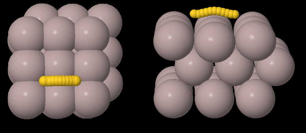
To demonstrate the basic functionality of the software, here we describe how an UV-Visible spectrum of a silver nanocluster can be calculated using DFTB+ code in conjunction with the DJMol software. There are three steps to calculate the spectrum, viz. (1) Obtain the structure of Ag nanocluster, (2) Optimize the structure and create the corresponding HSD file for the TD-DFTB calculation and, (3) Plot the convoluted Spectrum data. Note that we arbitrarily choose Ag177 nanocluster (its diameter is around 1.5 nm) for the TD-DFTB calculation. And the geometry of this cluster is generated by OpenMD package (in CygWin environment) by using experimental lattice constant of silver (4.08 A) and FCC lattice structure.
The following commands are used in the DJMol terminal to obtain the Cartesian coordinate data of the system:
cmd.exe /c  nanoparticleBuilder --latticeConstant=4.08 --radius=15 Ag.omd -o NP15.omd
cmd.exe /c  Dump2XYZ -i NP15.omd
The resultant coordinate data (XYZ file), can be visualized by DJMol program to generate a dftb_in.hsd file using the DFTB+ Script Writer tool with appropriate settings, for example, by adding a conjugate gradient method. See SetUp menu for this utility. This HSD file can be then used to generate an optimized Ag177 cluster by executing a DFTB+ calculation. It can be seen that this optimized cluster (See geo_end.xyz file for the data) is approximately spherical in symmetry. The optimized structure was again visualized and used in the Script Writer tool to make another HSD file to include instructions for Casida method (a TD-DFTB algorithm).
The essential part of this script is:
. .
ExcitedState = Casida {
    NrOfExcitations=100
    StateOfInterest=0
    Symmetry=singlet
    WriteTransitions=no
    WriteSPTransitions=yes
    WriteMulliken=no
    WriteCoefficients=no
    WriteEigenvectors=no
    WriteTransitionDipole=no
    OscillatorWindow=0.01
}
. . .
In all the DFTB calculation, we used hyb-0-2 parameter set is used for the silver atoms. This newly generated HSD file is submitted to a remote Linux machine using the SSH utility (See Extra menu in the tool bar) of the DJMol and after finishing the calculation a SPX output file was retrieved in the local machine, which contains the oscillator strengths of different electronic excitations. It was then plotted with UV-Vis spectrum from the Tool menu to obtain the spectrum of the molecule. A Lorentzian convolution (with 0.035 eV of full width at half maximum) is used to obtain the spectrum as shown in the Figure Below. Note that the absorption maximum wavelength (\(\lambda_{max}\)) is located around 440 nm i.e. around the indigo-blue region. By plotting molecular orbital energy levels (using MOLevels tool and with the detailed.out file) one can seen that the Fermi level is near to 3.9 eV and band gap of this cluster is negligibly small (See the inset figure in Fig. below). And it qualitatively indicates that \(Ag_{177}\) behaves like a semi-metal.
Different sized nanoparticles can be constructed by applying the above said method to study red shift property of the system. See the Figure below. Experimentally this is a known fact for the Agn system (By comparing \(\lambda_{max}\) values of clusters, we can seen that, \(\lambda_{max}\) shifts towards UV region if we increase the size of the nano clusters.). This can be qualitatively justified by particle in a box analogy. Note that the diameter of \(Ag_{177}\) is longer than that of the \(Ag_{13}\) so that its electron can move longer along its diameter (the box length). This will reduce its \(\Delta E\) values significantly (by increasing the size of the diameter of a silver cluster, a photon from the red region - a wavelength that corresponds to a lower energy - can cause an electronic excitation). For experimental UV-Vis spectra, see: https://www.sigmaaldrich.com/technical-documents/articles/materials-science/nanomaterials/silver-nanoparticles.html.
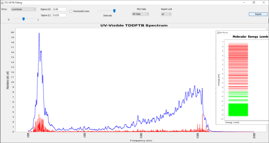
The UV-Visible spectrum of \(Ag_{177}\) nanocluster as it is plotted with the UV-Vis Spectrum tool. The vertical red line shows the oscillator strengths of electronic transitions. The inset figure shows HOMOs (green lines) and LUMOs (red lines) of the system.
Frontier Orbitals of C 60 Calculated with Siesta
Volumetric MO data can be made by using executing steps described in Denchar Utility, systematically using the Siesta add-on. The Siesta add-on can be invoked by:
Execute ➤ Siesta Calculator
In this section we shall obtain the frontier orbitals of Buckminster fullerene. See the example file Fullerene.fdf under the Siesta_Samples folder for its coordinate (note that it is an un-optimized structure; its optimization procedure is left to the user as an additional exercise). Since we used a molecular system in a unit cell, the default k-point (-point) is used to represent electronic wavefunction coefficients. Note that HOMO and LUMO coefficients are at 120 and 121’th k-points. See the Siesta Manual for more details. And change the main setting of the fdf file as (ie. except the coordinate as it is inserted between, AtomicCoordinatesAndAtomSpecies block):
#------------------------------------------------
#   IMPORTANT: DO NOT CHANGE SystemLabel
#------------------------------------------------


SystemName          Fullerene molecule        # Descriptive name of the system
SystemLabel         siesta                    # Short name for naming files

NumberOfAtoms       60
NumberOfSpecies     1

SpinPolarized               T

WriteDenchar                T
WriteWaveFunctions          T
COOP.Write                  T

%block WaveFuncKpoints
0.000 0.000 0.000 from 120 to 121            # Gamma wavefuncs Here, 120 = HOMO
%endblock WaveFuncKPoints

%block ChemicalSpeciesLabel
1  6  C                                       # SpeciesIndex,AtomicNumber,SpeciesLabel
%endblock ChemicalSpeciesLabel

LatticeConstant       25.0 Ang
%block LatticeVectors
1.0    0.0    0.0
0.0    1.0    0.0
0.0    0.0    1.0
%endblock LatticeVectors

AtomicCoordinatesFormat  Ang                   # Format for coordinates

%block AtomicCoordinatesAndAtomicSpecies
. . .
%endblock AtomicCoordinatesAndAtomicSpecies

WriteEigenvalues      T

#######################################################
# For the following parameters, default value is ok.
MeshCutoff               100. Ry       # Mesh cutoff. real space mesh (Ry)
PAO.BasisType            split         # Type of PAO basis set
PAO.EnergyShift          50 meV
PAO.BasisSize            DZ            # with polarization

# SCF options
MaxSCFIterations         60            # Maximum number of SCF iter

DM.MixingWeight          0.1           # New DM amount for next SCF cycle
DM.Tolerance             1.d-4         # Tolerance in maximum difference
                                    # between input and output DM
DM.NumberPulay           3
DM.UseSaveDM             F             # to use continuation files
MD.USeSaveXV             F

NeglNonOverlapInt        false         # Neglect non-overlap interactions

SolutionMethod           diagon        # OrderN or Diagon
ElectronicTemperature    6 K           # Temp. for Fermi smearing (Ry)

XC.Functional            GGA
XC.Authors               PBE
From this we can seen that, a double zeta type basis is used along with the PBE functional for the DFT calculation. A cubic box of 25 Å lengths is used to place the molecule.
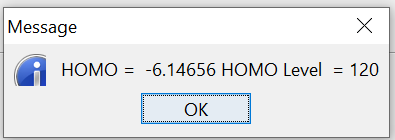
Run the calculation as usual and after finishing the run, plot MO energy levels, using MO Energies, which also indicate the level of HOMO (from the first occupied level, which is level 1):
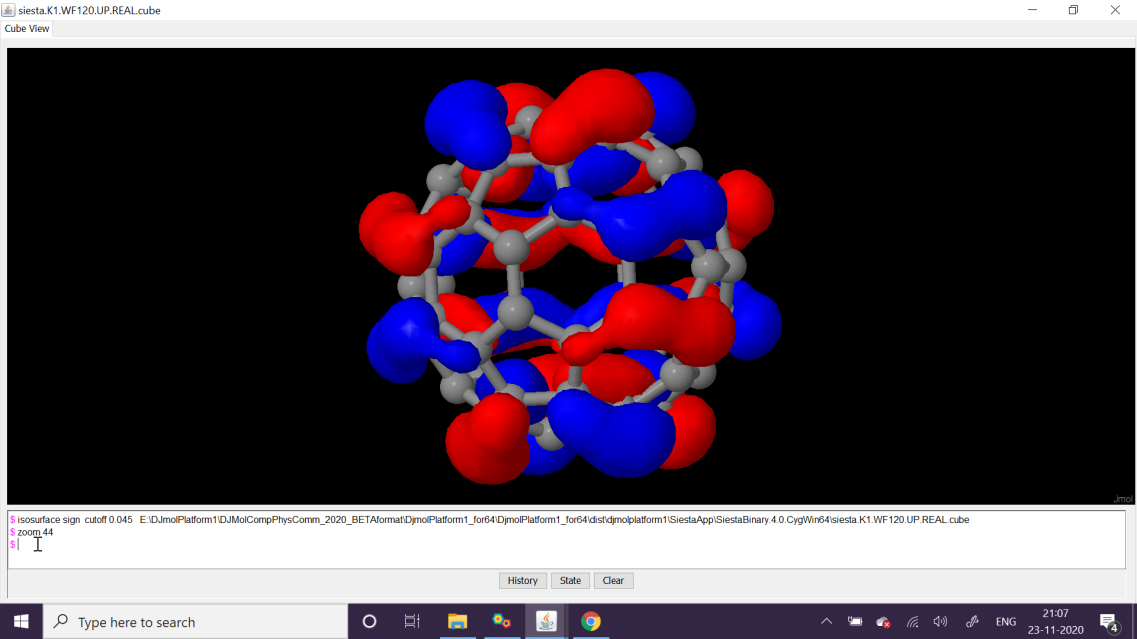
Then using, Edit denchar3D.fdf option insert the below text therein, and execute its next step, which is Run Denchar. After finishing View 2D/3D Files buttons can be clicked to view orbitals. Please see the next figures for the MOs of HOMO and LUMO (MO level, 120 and 121, respectively).
#------------------------------------------------
#   Note: It is a Sample Script only
#         You have to Modify this according
#         to your system/requirement
#     See the Manual for more details
#------------------------------------------------

Denchar.TypeOfRun                   3D

Denchar.PlotCharge                  T     # If .true. SystemLabel.DM   must be present
Denchar.PlotWaveFunctions           T     # If .true. SystemLabel.WFSX must be present

Denchar.CoorUnits       Ang
Denchar.DensityUnits    Ele/Ang**3

# set the mesh for wavefunction plot
Denchar.NumberPointsX 100
Denchar.NumberPointsY 100
Denchar.NumberPointsZ 100

Denchar.MinX          -12.5 Ang
Denchar.MaxX           12.5 Ang
Denchar.MinY          -12.5 Ang
Denchar.MaxY           12.5 Ang
Denchar.MinZ          -12.5 Ang
Denchar.MaxZ           12.5 Ang

%block ChemicalSpeciesLabel
1  6  C      # Species index, atomic number, species label
%endblock ChemicalSpeciesLabel
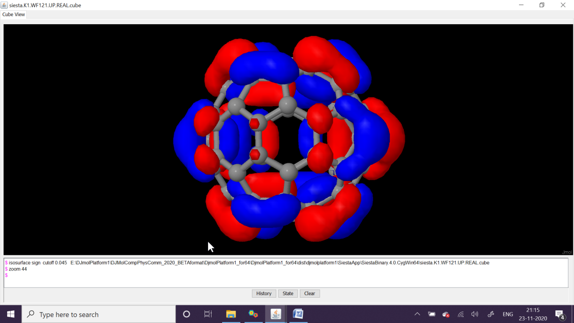
Using \(\Gamma\)-point Siesta’s SCF calculations yields MO coefficients. Here 120’th wavefunction at the -point (alias MO-120) is HOMO (upper figure) and MO-121 is LUMO. The qualities can be adjusted with Denchar parameter settings.
OpenMD MD simulation of Gold-nanoparticle
In this demonstration, we would obtain the gold-gold atom pair distribution function from the OpenMD molecular dynamics trajectory. One can open OpenMD tool by:
Execute ➤ OpenMD Tool
In first we have to construct a Au-nanoparticle (with icosahedron symmetry). A basic starting script for the calculation is given below (its file name is gold.omd, and note HTML styled tags in it)
<OpenMD>
<MetaData>

molecule{
name = "Au";

atom[0]{
type = "Au";
position(0.0, 0.0, 0.0);
    }
}

component{
type = "Au";
nMol = 1;
}

forceField = "SC";
forceFieldFileName = "SuttonChen.QSC.frc";

</MetaData>
</OpenMD>
Using the command (in the OpenMD tool’s command shell window) save the file, gold.omd ,with the above data.
cmd.exe /c notepad.exe gold.omd
Then run the following commands one after another:
cmd.exe /c .icosahedralBuilder.exe -o file.omd –shell=8 –latticeConstant=4.08 –ico gold.omd
cmd.exe /c Dump2XYZ -i file.omd
cmd.exe /c more file.xyz
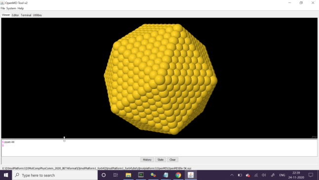
If everything is correct you will get a gold-nanoparticle structure as shown in the below figure-a. The above procedure construct a file called, file.omd which contains all the XYZ data of the nanoparticle. However in order to start an MD run, we need initial velocities. For the purpose please run the command:
cmd.exe /c .thermalizer -t 5 -o file-5K.omd file.omd
It will create a new file, file-5K.omd with new initial velovities and 5 Kelvin as its target temperature. Its main parameters are:
forceField = "SC";
forceFieldFileName = "SuttonChen.QSC.frc";

ensemble = "LHull";
targetTemp = 5;
targetPressure = 1;
viscosity = 0.1;

dt = 2.0;
runTime = 2E5;
sampleTime = 500.0;
statusTime = 4;
seed = 985456376;
usePeriodicBoundaryConditions = "false";
tauThermostat = 1E3;
tauBarostat = 5E3;
Then run the actual OpenMD molecular dynamics run as,
cmd.exe /c openmd file-5K.omd
This may take a while (2 hour), and its trajectory information will stored in the dump file. From this MD animation can be retrived as:
cmd.exe /c Dump2XYZ -b -i file-5K.dump
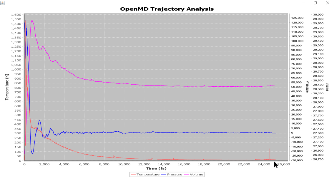
Moreover, from the below figure one can see that the 5K thermalization is achieved in the MD run (note its convergence to 5K)
After that, a script utility to retrieve, \(g_{Au-Au}(r)\), as
cmd.exe /c StaticProps.exe -i file-5K.dump –gofr –sele1=”select Au* –sele2=”select Au*”
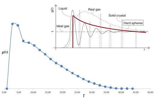
Pair correlation function (g(r)) obtained from the MD trajectory data which use only test-level parameters. Note the similarity with g(r) obtained by a hard-sphere model (inset figure courtesy, J. Nanopart. Res, 13, 4277 (2011).)
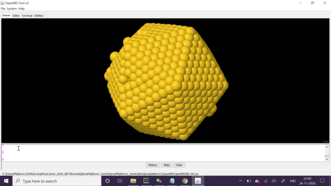
The initial (top) and final (bottom) snapshot of the MD run. Note that the system’s initial temperature was 0K and it was equilibrated to 5K during the MD run.
ASE simulation of an adatom diffusion
Here we use ASE to obtain the energy profile of a physical process - diffusion of an adatom or adsorbed atom (Au) on the top of a metallic surface of Al atoms. Nudged elastic band (NEB) method is used for the calculation, in which an initial structure (where an adatom i.e. gold atom is placed in the left side) and a final structure (adatom is placed in the right side) of the process is used as its input data. For more details please visit ASE tutorial web page. Note that we used EMT calculators (it is a really fast albeit highly approximated potential function) for this calculation however one can use Siesta within ASE to obtain more realistic diffusion barrier.
Refer Chapter-5 for creating a Python Project. Then add an Empty module (InitialFinalStructure.py fie) into the src directory. Then add the following Python source into it:
from ase.build import fcc100, add_adsorbate
from ase.constraints import FixAtoms
from ase.calculators.emt import EMT
from ase.optimize import QuasiNewton

# 3x3-Al(001) surface with 3 layers and an
# Au atom adsorbed in a hollow site:
slab = fcc100('Al', size=(3, 3, 3))
add_adsorbate(slab, 'Au', 1.7, 'hollow')
slab.center(axis=2, vacuum=4.0)

# Fix second and third layers:
mask = [atom.tag > 1 for atom in slab]
slab.set_constraint(FixAtoms(mask=mask))

# Use EMT potential:
slab.calc = EMT()

# Initial state:
qn = QuasiNewton(slab, trajectory='initial.traj')
qn.run(fmax=0.05)

# Final state:
slab[-1].x += slab.get_cell()[0, 0] / 3
qn = QuasiNewton(slab, trajectory='final.traj')
qn.run(fmax=0.05)
Then Run the file (Run ► Run File). This will create, initial.traj and final.traj files which contains the initial and final structure respectively.
After this, the NEB calculation can be started (don’t forget to create a new Python file for this) and its Python source is given below:
# To change this license header, choose License Headers in Project Properties.
# To change this template file, choose Tools | Templates
# and open the template in the editor.
from ase.io import read
from ase.constraints import FixAtoms
from ase.calculators.emt import EMT
from ase.neb import NEB
from ase.optimize import BFGS

initial = read('initial.traj')
final = read('final.traj')

constraint = FixAtoms(mask=[atom.tag > 1 for atom in initial])

images = [initial]
for i in range(9):
    image = initial.copy()
    image.calc = EMT()
    image.set_constraint(constraint)
    images.append(image)

images.append(final)

neb = NEB(images)
neb.interpolate()
qn = BFGS(neb, trajectory='neb.traj')
qn.run(fmax=0.05)
The energy profile can be saved in a PNG image by using the following script:
import matplotlib.pyplot as plt
from ase.neb import NEBTools
from ase.io import read

images = read('neb.traj@-11:')

nebtools = NEBTools(images)

# Get the calculated barrier and the energy change of the reaction.
Ef, dE = nebtools.get_barrier()

# Get the barrier without any interpolation between highest images.
Ef, dE = nebtools.get_barrier(fit=False)

# Get the actual maximum force at this point in the simulation.
max_force = nebtools.get_fmax()

# Create a figure like that coming from ASE-GUI.
fig = nebtools.plot_band()
fig.savefig('diffusion-barrier.png')

# Create a figure with custom parameters.
fig = plt.figure(figsize=(5.5, 4.0))
ax = fig.add_axes((0.15, 0.15, 0.8, 0.75))
nebtools.plot_band(ax)
fig.savefig('diffusion-barrier.png')
Finally, the neb.traj file, which contains the entire geometry of the process in binary format, is then used to obtain XYZ format by the following script:
import matplotlib.pyplot as plt
from ase.calculators.emt import EMT
from ase.neb import NEB
from ase.optimize import BFGS
from ase.io import read, write
import os

# read the last structures (of 5 images used in NEB)
images = read('neb.traj@-11:')

for i in range(0,  len(images)):
    atoms = images[i]
    #print(atoms.get_positions())
    write('delete.xyz', atoms)
    inFile = open(os.path.join( 'delete.xyz'), 'r')
    fileStr = inFile.read()
    outFile = open("neb_movie.xyz", 'a')
    outFile.write(fileStr)

# @type outFile
outFile.close()
inFile.close()
Additionally, using DJMol’s xyz File loader (File►Open Structure) the geometries of the process as it is saved in “neb_movie.xyz” can be displayed or animated (See the below figure).

Starting (I) and ending (F) geometries of the Diffusion of gold atom; The diffusion barrier (around 0.35 eV) is shown in the inset.
